Every location on Earth has its own unique perspective. Azimuthal projections reveal that perspective, showing the world as seen from your chosen center. This tool offers two projection types: the azimuthal equidistant, which preserves spherical distances and initial directions from the center (ideal for navigation and radio bearings), and the Lambert azimuthal equal-area, which preserves the relative sizes of all regions (ideal for thematic maps and comparing areas). Whether you're a ham radio operator, a cartographer creating statistical maps, or simply curious about what's on the opposite side of the world, generate a custom map centered on your location.

Azimuthal Map Generator

Width & height of exported image

Loading map data...

Center: 0.0000°, 0.0000°

Width & height of exported image

Loading map data...

Center: 0.0000°, 0.0000°

Understanding Azimuthal Projections

Azimuthal projections arrange the map around a chosen center point. In their spherical forms, they preserve initial direction from that center, except at the antipode where direction is undefined. What differs among azimuthal projections is what else they preserve.

Property Azimuthal Equidistant Lambert Equal-Area
Distance from center Accurate Distorted
Initial direction from center Accurate on sphere* Accurate on sphere*
Area Distorted Accurate everywhere
Shape Distorted at edges Distorted at edges
Great circles as straight lines Those through center Those through center
Best for Navigation, radio bearings, distance analysis Thematic maps, statistical mapping, area comparison

* Direction is undefined at the antipode.

Azimuthal Equidistant Projection

The azimuthal equidistant projection preserves two critical properties from the center point:

  • Distance: The straight-line distance on the map from the center to any other point equals the true great-circle distance on Earth.
  • Direction: The angle from the center gives the initial great-circle azimuth to any point except the antipode.

This makes it invaluable for applications where you need to know "how far?" and "which way?" from a specific location. The name comes from azimuth (a direction measured as an angle from north) and equidistant (equal distances preserved from the center).

Great Circle Navigation (Equidistant)

USGS diagram showing azimuthal equidistant projection with plane of projection

Image: USGS

A key property of the equidistant projection: any straight line drawn through the center point lies on a great circle, the shortest path between two points on a sphere. This is why the projection is so valuable for aviation and radio: draw a straight line from the map center to a destination to trace the spherical great-circle route.

See Interactive Animation

Video: A Quick Overview of the Azimuthal Equidistant Projection
Video Transcript

When mapping the world from a single point, how do you keep distances accurate? This is the azimuthal equidistant projection.

Centered on a chosen location, an azimuthal equidistant map shows every other point at its spherical great-circle distance and initial azimuth from that center, except that direction is undefined at the antipode. Imagine stretching the globe out radially from that point — distances from the center stay correct, while transverse distortion increases outward.

Take a look at this animation. At the top is a 3-D globe and at the bottom an azimuthal equidistant map centered at the same point. Each colored spoke is a meridian; follow any spoke outward from the center and you'll see that the radial distance on the flat map equals the true great-circle distance from the center on the globe. When a point falls on the globe's far side it becomes hidden in the globe view — and it is also not shown on the flat projection. The set of points that remain visible on the projection therefore provides a clear frame of reference for what the globe is currently displaying.

You can use this projection when you need accurate bearings or ranges from one site. For example: radio planning, expedition maps, or local route planning. But remember: distances between two non-central points are not preserved, and shapes can distort near the rim, and the antipode can smear into a ring.

To learn more about azimuthal projections and generate your own custom maps, you can visit azimuthalmap.com.

Lambert Azimuthal Equal-Area Projection

The Lambert azimuthal equal-area projection, presented by Swiss mathematician Johann Heinrich Lambert in his 1772 treatise Beiträge zum Gebrauche der Mathematik und deren Anwendung, preserves a different property:

  • Area: All regions on the map are shown at their correct relative size. A country that's twice the size of another will appear twice as large, regardless of where they are on the map.
  • Direction: In the spherical form used here, initial directions from the center are true except at the antipode.

Lambert called this a "synthetic" azimuthal projection. It is not a perspective projection (you cannot create it by shining light through a globe), but rather is constructed mathematically to ensure equal area. The projection is widely used for thematic mapping, statistical analysis, and continental atlases where comparing the sizes of regions matters more than measuring distances. (USGS PP1395, Wikipedia)

Area Preservation (Equal-Area)

USGS diagram showing Lambert azimuthal equal-area projection

Image: USGS

As with other azimuthal projections, great circles through the center appear as radial straight lines. Other great circles are generally curved; only the gnomonic projection makes every great circle straight. The equal-area property makes Lambert useful for statistical maps, density visualizations, and any application where accurate area comparison is essential.

What These Projections Are Not

Neither projection is conformal: they do not preserve local shapes and angles (like the stereographic projection does). Neither is a perspective projection: you cannot create either by projecting light through a globe onto a plane. Both are constructed mathematically to achieve their specific properties.

The fundamental trade-off in cartography: no flat world map can preserve both area and angles everywhere. The equidistant projection preserves distance from its center (at the expense of area), while the equal-area projection preserves area (at the expense of distance). Choose based on what property matters most for your application. (USGS PP1395)

The Three Aspects

Both azimuthal projections can be centered anywhere on Earth. Cartographers categorize them into three aspects based on where the projection plane touches the globe. Lambert's 1772 paper discussed the polar and equatorial aspects; the oblique aspect is equally popular today for location-specific maps.

Polar aspect: projection centered on North or South Pole
Polar Centered on North or South Pole. Parallels appear as concentric circles; meridians as straight radial lines.
Oblique aspect: projection centered on any point except poles or equator
Oblique Centered on any point except poles or equator. Most flexible; used for location-specific maps.
Equatorial aspect: projection centered on the equator
Equatorial Centered on the equator. Often used for hemisphere maps in atlases.

Related Azimuthal Projections

The azimuthal equidistant and Lambert equal-area are part of the azimuthal family. All are centered on a single point, but each preserves different properties:

Azimuthal Equidistant Preserves distance from center
Lambert Azimuthal Equal-Area Preserves relative area
Stereographic Preserves local shapes and angles
Gnomonic Shows all great circles as straight lines
Orthographic View from infinite distance (like a photograph from space)

Beyond single-center projections: The Two-Point Equidistant projection preserves distances from two chosen points. The Hammer projection (1892) is a modification of Lambert's equal-area that shows the entire world in an ellipse, created by halving vertical coordinates and doubling meridian values.

Practical Applications

Azimuthal projections solve real problems where understanding spatial relationships from a specific point matters. Choose the equidistant projection when distance and direction are critical; choose equal-area when comparing region sizes.

Equidistant Projection Applications

Ham Radio & Antennas

Radio operators use azimuthal maps centered on their station to determine the initial great-circle bearing for directional antennas. Point your beam antenna along the azimuth line to the target station for optimal signal strength.

Aviation & Navigation

Great-circle routes (the shortest paths between two points on a sphere) appear as straight lines radiating from the center. Pilots and navigators use these maps to plan fuel-efficient long-haul flights.

Seismology

Seismologists center maps on earthquake epicenters to visualize how seismic waves propagate outward. The concentric distance rings show which cities fall within different impact zones.

Defense & Range Analysis

Military analysts use azimuthal maps to visualize missile ranges, radar coverage, and strike capabilities. The famous North Korea missile range map uses this projection with concentric circles showing different missile capabilities.

Telecommunications

Satellite ground stations and telecommunications planners use azimuthal projections to determine coverage areas and signal paths from transmission points.

Emergency Response

First responders can visualize evacuation radii, response times, and resource deployment distances from an incident location, all accurately represented on a single map.

Equal-Area Projection Applications

Statistical Mapping

The European Environment Agency uses the Lambert azimuthal equal-area projection (ETRS89-LAEA) as the standard for European statistical and analytical mapping, ensuring accurate area comparisons across the continent.

Continental & Hemisphere Maps

Commercial atlases like The Times Atlas of the World use Lambert equal-area for continental maps where accurate size comparison matters. It's common for Eastern/Western hemisphere maps in educational materials. (Wikipedia)

Geology & Structural Analysis

Geologists use Schmidt nets, equal-area stereonets based on this projection, to plot crystallographic axes, foliation, lineation in rocks, and fault orientations. Wulff nets instead use the stereographic, equal-angle projection.

Thematic Mapping

Any map showing density, distribution, or comparative data (population, climate, resources) benefits from equal-area projection. Accurate area ensures visual data representation isn't skewed by projection distortion.

Polar Region Mapping

The USGS National Atlas uses Lambert equal-area for polar expedition maps at 1:39,000,000 scale and Arctic hydrocarbon maps at 1:20,000,000 scale. (USGS PP1395)

Ocean Basin Mapping

The USGS has prepared six Pacific Ocean base maps using Lambert equal-area at scales from 1:8,300,000 to 1:17,100,000, used for geologic, tectonic, and energy resource mapping. (USGS PP1395)

Famous Examples

Equidistant Projection Examples

United Nations Flag featuring azimuthal equidistant projection

The United Nations Emblem

The UN flag features a polar azimuthal equidistant projection centered on the North Pole, extending to 60° south latitude. Adopted in 1946, it symbolizes a unified global perspective: no single nation is placed at the center or given visual prominence over others.

Polish amateur radio station SP1QE with a 1930s vacuum tube transmitter and receiver

Ham Radio Beam Heading Maps

Amateur radio operators use azimuthal equidistant maps centered on their home location to aim directional antennas. The map shows the initial great-circle bearing toward any location except the antipode, supporting long-distance (DX) communication planning.

Star chart showing constellations using polar projection

Star Charts & Planispheres

Polar projections are ideal for mapping the night sky. While stereographic projection is most common (preserving constellation shapes), the azimuthal equidistant is also used in planispheres, rotating star wheels that show which stars are visible at any date and time. (Image: d3-celestial)

Equal-Area Projection Examples

European Environment Agency reference grid based on ETRS89-LAEA projection

European Environment Agency Grid

The ETRS89-LAEA (Lambert Azimuthal Equal-Area) is the official projection for European statistical mapping. The European Environment Agency mandates its use for pan-European spatial analysis, ensuring accurate area comparisons across all member states. (Image: EEA)

Logo of the National Atlas of the United States

National Atlas of the United States

The National Atlas online Map Maker application uses Lambert azimuthal equal-area for displaying information, as do USGS polar expedition maps (1:39,000,000) and Arctic hydrocarbon province maps (1:20,000,000). (USGS PP1395)

Schmidt net (stereonet) used in structural geology for plotting orientations

Schmidt Net (Stereonet)

The Schmidt net is a fundamental tool in structural geology, based on the Lambert equal-area projection. Geologists use it to plot orientations of crystallographic axes, fault planes, and rock formations. The equal-area property enables statistical analysis of directional data. (Image: Wikipedia)

Understanding Distortion

No flat map can perfectly represent a sphere, so something must be sacrificed. Both azimuthal projections prioritize different properties, but each trades off other characteristics as angular distance from the center increases.

Equidistant Projection Distortion

The azimuthal equidistant projection preserves distance and direction from the center only. Area and shape experience increasing distortion toward the edges.

0 – 5,000 km Lower Near the Center

Distortion starts at zero at the center and increases continuously. At about 5,000 km (45°), transverse scale is already about 1.11.

5,000 – 10,000 km Increasing Distortion

Tangential stretching becomes conspicuous. At about 10,000 km (90°), transverse scale is about 1.57, and the enclosed spherical cap is a hemisphere: half Earth's surface.

10,000 – 20,000 km Strong to Extreme Distortion

Transverse stretching grows rapidly and becomes unbounded toward the antipode, which maps around the outer boundary.

The Antipode Effect

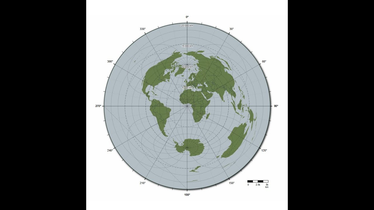
On a spherical Earth model, the maximum distance on an azimuthal equidistant map is half a great-circle circumference, about 20,000 km. At this distance, a single point (the antipode) gets stretched into the entire outer circle of the map. This is why Antarctica appears as a ring when the map is centered on the Arctic.

Curious about what's on the opposite side of the world from you? Check out Antipode Finder, where you can explore antipodal points using multiple map projections, including azimuthal views.

Equal-Area Projection Distortion

The Lambert azimuthal equal-area projection preserves area everywhere on the map, making it ideal for density comparisons and statistical analysis. However, angular distortion (shape warping) increases with distance from the center.

Entire Map Area Preserved

Relative area is preserved throughout the projection, including beyond 90° from the center.

45° – 90° Increasing Angular Distortion

Shapes become increasingly compressed radially and stretched tangentially. Circles become ellipses, but their areas remain correct.

At Antipode Maximum Shape Distortion

The single antipodal point is represented around the 180° outer boundary. Radial scale tends to zero while transverse scale becomes unbounded.

Quantifying Angular Distortion

Maximum angular deformation ω can be calculated from the local radial and transverse scale factors. At 90° from the center, halfway to the 180° antipodal boundary, it is about 39°. The relationship is:

sin(ω/2) = |kt - kr| / (kt + kr)

where kr and kt are the radial and transverse scale factors. (USGS PP1395, p. 182)

Choosing the Right Projection

Your choice between equal-distance and equal-area depends on what you need to show:

  • Use Equidistant when measuring distances or showing travel routes from a specific location: radio propagation, flight paths, or missile ranges.
  • Use Equal-Area when comparing sizes, showing density distributions, or performing statistical analysis: population density, climate data, or ecological surveys.
  • Center near your region of interest for both projections to keep it in the low-distortion zone.
  • For global views, polar centers or mid-ocean centers often produce the least visually jarring results.

A Brief History

Ancient

Early use for star maps in Egyptian astronomical texts.

1025 CE

Abu Rayhan Biruni produces the earliest known mathematical description of the azimuthal equidistant projection in his treatise on cartography.

1426

Conrad of Dyffenbach creates the earliest known polar azimuthal equidistant map of the world's land masses. (USGS PP1395)

1510

Heinrich Glarean creates the earliest surviving terrestrial map using this projection, a pair of hemispheres. (Robles Macías, 2024)

1569

Gerardus Mercator includes a polar azimuthal equidistant inset in his famous world map.

1581

Guillaume Postel publishes a world map using this projection. In France and Russia, it's still called the "Postel projection" in his honor.

1772

Johann Heinrich Lambert publishes Anmerkungen und Zusätze zur Entwerfung der Land- und Himmelscharten (Notes and Additions on the Composition of Terrestrial and Celestial Maps), introducing the Lambert azimuthal equal-area projection along with several other projections still in use today. (USGS PP1395, p. 182)

1880s

French cartographer Philippe Hatt develops ellipsoidal versions of the oblique aspect, later adopted by France and Greece for coastal and topographic mapping. (USGS PP1395)

1946

The United Nations adopts a polar azimuthal equidistant projection for its emblem and flag.

Today

Both projections are used worldwide. The equidistant version dominates in radio communications, aviation planning, and seismology. The equal-area version is the standard for statistical mapping, including the ETRS89-LAEA projection used across the European Union. Both are available in PROJ, GeographicLib, and all major mapping platforms.

Mathematical Formulas

The azimuthal equidistant projection maps a point on the sphere with latitude $\varphi$ and longitude $\lambda$ to Cartesian coordinates $(x, y)$ on a plane, centered at $(\varphi_0, \lambda_0)$.

Distance from Center (ρ)

The arc distance from the center point to any other point:

$$\cos\left(\frac{\rho}{R}\right) = \sin\varphi_0 \sin\varphi + \cos\varphi_0 \cos\varphi \cos(\lambda - \lambda_0)$$

Where $R$ is the Earth's radius (~6,371 km).

Azimuth Angle (θ)

The compass direction from the center point:

$$\theta = \operatorname{atan2}\left(\cos\varphi \sin(\lambda - \lambda_0),\; \cos\varphi_0 \sin\varphi - \sin\varphi_0 \cos\varphi \cos(\lambda - \lambda_0)\right)$$

Cartesian Coordinates

Converting polar coordinates $(\rho, \theta)$ to $(x, y)$:

$$x = \rho \sin\theta, \qquad y = \rho \cos\theta$$

Simplified Polar Case

When centered on the North Pole ($\varphi_0 = 90°$), the formulas simplify to:

$$\rho = R\left(\frac{\pi}{2} - \varphi\right)$$ $$x = \rho \sin(\lambda - \lambda_0), \qquad y = -\rho \cos(\lambda - \lambda_0)$$

Radial distance is proportional to co-latitude; longitude determines position around the polar map.

Sphere vs. Ellipsoid

These formulas assume a perfect sphere. For precision applications, the Earth is better modeled as an ellipsoid (WGS84). Libraries like GeographicLib provide ellipsoidal corrections. For most visualization purposes and distances under a few thousand kilometers, spherical calculations are sufficiently accurate.

Lambert Azimuthal Equal-Area Formulas

The Lambert azimuthal equal-area projection also maps points to Cartesian coordinates, but uses a different radial scaling to preserve area rather than distance. (USGS PP1395, pp. 182-190)

Forward-Equation Coefficient (k')

The Cartesian-coordinate equations use the following coefficient:

$$k' = \sqrt{\frac{2}{1 + \sin\varphi_0 \sin\varphi + \cos\varphi_0 \cos\varphi \cos(\lambda - \lambda_0)}}$$

This coefficient is not the local radial scale. At angular distance $c$ on the spherical projection, radial scale is $k_r = \cos(c/2)$ and transverse scale is $k_t = \sec(c/2) = k'$. Their product is 1, preserving area.

Cartesian Coordinates

Converting spherical to planar coordinates:

$$x = R \cdot k' \cos\varphi \sin(\lambda - \lambda_0)$$ $$y = R \cdot k' \left[\cos\varphi_0 \sin\varphi - \sin\varphi_0 \cos\varphi \cos(\lambda - \lambda_0)\right]$$

Simplified Polar Case

When centered on the North Pole ($\varphi_0 = 90°$), the formulas simplify to:

$$\rho = 2R \sin\left(\frac{90° - \varphi}{2}\right)$$ $$x = \rho \sin(\lambda - \lambda_0), \qquad y = -\rho \cos(\lambda - \lambda_0)$$

Compared with the equidistant case, radial spacing is increasingly compressed away from the center while transverse scale expands, preserving area.

Inverse Formulas

To convert from map coordinates back to latitude and longitude:

$$\varphi = \arcsin\left(\cos c \sin\varphi_0 + \frac{y \sin c \cos\varphi_0}{\rho}\right)$$ $$\lambda = \lambda_0 + \operatorname{atan2}\left(x \sin c,\; \rho \cos\varphi_0 \cos c - y \sin\varphi_0 \sin c\right)$$

Where $\rho = \sqrt{x^2 + y^2}$ and $c = 2 \arcsin\left(\frac{\rho}{2R}\right)$.

Frequently Asked Questions

An azimuthal equidistant projection preserves spherical distances from a chosen center point and initial azimuths from that center, except at the antipode where direction is undefined. The name comes from "azimuth" (a direction measured as an angle from north) and "equidistant" (equal distances are preserved from the center).

Spherical distances and initial directions from the center are preserved, except that direction is undefined at the antipode. Distances between two points where neither is the center are generally distorted:

  • Near the center: Distortion starts at zero and increases continuously outward
  • At about 5,000 km (45°): Transverse scale is about 1.11
  • At about 10,000 km (90°): Transverse scale is about 1.57
  • Near 20,000 km (180°): Transverse scale becomes unbounded at the antipode

On a North-Pole-centered map, Antarctica lies near the outer boundary and the South Pole is the exact antipode, about 20,000 km from the center on a spherical model. That single antipodal point is represented around the entire outer boundary. This isn't an error; it's a mathematical consequence of the projection. Antarctica appears normally on maps centered in the Southern Hemisphere.

Only if one of those cities is the map's center point. The azimuthal equidistant projection preserves distances from the center only. To find the accurate distance between two arbitrary cities, you would need to generate a new map centered on one of them, or use a great-circle distance calculator.

Azimuth is measured clockwise from true north (geographic north pole), ranging from 0° to 360°. Compass bearing often references magnetic north, which differs from true north by the local magnetic declination. Standard azimuthal maps reference true north unless their orientation states otherwise. If you're using a magnetic compass to follow directions from an azimuthal map, you'll need to apply the appropriate declination correction for your location.

No. The azimuthal equidistant projection is derived from spherical geometry and is mathematically dependent on Earth being a sphere (or ellipsoid). The distortion patterns, especially the antipodal smearing, are exactly what spherical trigonometry predicts. The UN flag uses this projection not because the Earth is flat, but because the polar view treats all nations equally around the center. Ironically, the projection's distortion characteristics are evidence of Earth's curvature, not an alternative to it.

On a spherical Earth model, a great-circle circumference is approximately 40,000 km. The farthest any point can be from the center along the surface is half that distance: the antipodal point, about 20,000 km away. Going any "farther" would actually bring you closer again from the other direction. This is why azimuthal equidistant maps have a natural circular boundary at roughly 20,000 km radius.

Equal-Area Projection Questions

The Lambert azimuthal equal-area projection is a map projection that preserves area everywhere on the map. Any region on the map has the correct size relative to any other region. It was invented by Johann Heinrich Lambert in 1772 and is widely used for statistical mapping, thematic maps, and scientific analysis where accurate area representation matters.

Use equal-area when comparing sizes or showing density data: population maps, climate data, election results, or ecological surveys. Use equidistant when measuring distances or showing routes from a specific point: radio coverage, flight paths, or seismic distances. Neither is "better"; they serve different purposes.

Yes. Because it preserves area, shapes must be distorted to compensate. This is a fundamental trade-off in cartography. Near the center, shapes are nearly correct. Moving outward, features become compressed radially and stretched tangentially. The distortion is most severe at the map's edge, where shapes can appear significantly flattened.

The European Terrestrial Reference System 1989 Lambert Azimuthal Equal-Area (ETRS89-LAEA) projection is the official standard for statistical mapping across the European Union. It's centered at 52°N, 10°E (roughly central Germany) and uses the EPSG:3035 coordinate reference system. The equal-area property enables accurate comparison of statistics across member states.

A Schmidt net is a graphical tool used by geologists to plot and analyze three-dimensional orientation data on a two-dimensional surface. It's based on the Lambert azimuthal equal-area projection, which ensures that clusters of data points reflect true density distributions. Geologists use it to analyze rock structures, fault orientations, and crystallographic data.